Dissolution Theory

 

ã Copyright 2011 by Alex Avdeef. All rights reserved.   

 

This section is a rigorous theoretical discussion of the state-of-the-art data analysis used for interpreting pH-dependent dissolution processes exhibited by poorly-soluble multiprotic ionizable test compounds synthesized by medicinal chemists in pharmaceutical companies.^1-5 This data analysis is encoded in the µDISS-X software from in‑ADME Research.

 

This can be of interest to candidate-selection analytical/physical chemists intent on designing information-rich dissolution measurements, and on effectively communicating these results to medicinal chemists, so that rational structural modifications leading to improved physicochemical properties can be made.  Also, this can be of interest to preformulation scientists, charged downstream with the daunting task of formulating very insoluble molecules into drug products.

 

The enhanced theory of dissolution kinetics is spotlighted with the convective diffusion & simultaneous chemical reaction (CDR) model, incorporating the low-ionic-strength Vinograd-McBain⁶ electric field treatment.  The new computational treatment described here extends the generality and robustness of the CDR model, clarifies limitations in earlier underlying assumptions, and aspires to provide some of the finishing touches to the pioneering works of Higuchi et al.,^15,16  Mooney et al.,^17-20 McNamara et al.,^21-23 and Southard et al.,²⁴ and a number of others. 

 

The coverage here is focused on two applications of CDR data analysis: (a) rotating disk intrinsic dissolution rate (disk-IDR)²⁵ and (b) Wang-Flanagan ^7,8 spherical particle model (particle-IDR) models.  The rigorous CDR kinetics model may be most helpful in early applications of IDR, where compounds are studied as compacted solid rotating disks or suspended powders of the pure compound.  Such investigations are done long before the traditional formulation development and quality control type of applications.

 

Concentration-time profiles as a function of pH, buffers, salt, complexation and self-aggregation are considered.  Concentration-position profiles of all species in the aqueous boundary layer (ABL), including solid species, are also considered under the above conditions.  The new small-volume (≥ 1 mL) dip-probe UV detection apparatus, developed by pION INC for polymorph transformation/salt selection/solubility screening, is discussed using published case studies.^9-14 

 

 

Noyes-Whitney Model, its Mooney Extension, and the Dissolution Titration

 

The relationship between the rate of dissolution, dm/dt, and the solubility, C_S, is described by the Noyes-Whitney²⁶ equation

 

                                 dm/dt = A∙(D/h_ABL)∙(C_S - C)                                                                         (1)

 

where m = mass (mol), t = time (s), C = concentration of solute dissolved at a particular time (mol∙cm^–3), C_S = equilibrium solubility (mol∙cm^–3), D = diffusivity (cm²∙s^–1) , h_ABL = apparent thickness (cm) of the aqueous boundary layer (depends on rate of stirring and the temperature), and A = surface area available for dissolution (cm²). 

 

According to the Nernst-Brünner diffusion layer model,^27,28  the outermost layer of the solid compound dissolves very quickly into a thin layer of solvent to form a saturated solution adjacent to the surface, and a steady state of material flows into the bulk solution.  For diffusion layer thickness of 10 - 100 mm and drug diffusivities about 5 x 10^-6 cm² s^–1, the time to reach steady state is under 2 s.²⁹  When dissolving ionizable compounds undergo simultaneous chemical reactions, such as ionization, Eq. 1 needs to be expanded.  The rate can depend dramatically on the pH of the test solution, on the presence of buffers, complexing agents, and excipients.

 

In their comprehensive work with the dissolution kinetics of ionizable weak acids, Mooney et al.^17‑20 have developed critical extensions of the Noyes-Whitney equation.  It was necessary to consider the concentrations of species in the diffusion layer (ABL), at the solid-liquid interface, rather than solely in the bulk solution in order to rationalize the observed dissolution.  McNamara et al.^21-23 introduced to the evolving treatment the effects of convection, using a dimensionless variable approach described earlier by Litt and Serad.³⁰  Southard et al.²⁴ considered a numerical integration in their CDR method.  McNamara et al.⁴ reviewed the early efforts, citing computational challenges, shortcomings, and incremental advances: “Today, the opportunity is still available, for those inclined to numerical analysis, to derive a robust numerical dissolution model capable of including contributions due to diffusion, convection, and reaction which can encompass the entire pH scale…”   

 

To explore the dynamics of dissolution processes, one can begin with the steady-state kinetics model of Mooney and coworkers.  Consider the system of reactions of a weak base, as a function of pH.  The corresponding mass balance equations in the aqueous phase are

 

                                 [B]_total = [B] + [BH⁺]                                                                                 (2a)

                                 [H]_total = [H⁺] – [OH ^–] + [BH⁺]                                                                    (2b)

 

[B]_total and [H]_total are the total concentrations of the weak base and the hydrogen excess, respectively, as functions of position x and time t.  From Fick’s first law of diffusion, the steady-state flux (mol∙cm^–2∙s^–1) is

 

                                J =  – D∙(dC/dx)  =  (dm/dt)∙/A  = (V/A)∙(dC/dt)                                         (3)

 

The solutions to the differential expressions, Eqs. 2 applied to Eq. 3, can be stated as¹⁷

 

                                 D_B [B] + D_BH [BH⁺] = c₁ x + c₃                                                                    (4a)

                                 D_H [H⁺] – D_OH [OH ^– ] + D_BH [BH⁺] = c₂ x + c₄                                                (4b)

 

with integration constants c₁ to c₄.  The D-terms refer to diffusivities of the various reactants. Two sets of boundary concentrations need to be considered to solve the above equations.  One set consists of all of the equilibrium reactant concentrations at x=0, in the diffusion layer adjacent to the surface of the solid, and another set consists of reactant concentrations at x ³ h_ABL (bulk solution).  The former set is labeled [B]_o, [BH⁺]_o, [H⁺]_o, and [OH ^–]_o, while the latter set is labeled [B]_h, [BH⁺]_h, [H⁺]_h, and [OH ^–]_h.  Substitutions of the boundary conditions into Eqs. 4 eliminate some of the integration constants to produce

 

                                 c₁ = – { D_B ([B]₀ – [B]_h)/h + D_BH ([BH⁺]₀ – [BH⁺]_h)/h }                                     (5a)

                                 c₂ = - { D_H ([H⁺]₀ – [H⁺]_h)/h - D_OH ([OH^–]₀ - [OH^–]_h)/h + D_BH ([BH⁺]₀ - [BH⁺]_h)    (5b)

 

The initial total flux of the dissolving substance is expressed by Eq. 5a.  One can make the approximation that D_B» D_BH¹⁷ and obtain the initial-state dissolution flux expression

 

                                (dm/dt) / A  = (D_B/h_ABL)∙( [B]₀ – [B]_h + [BH⁺]₀ – [BH⁺]_h )

                                             = (D_B/h_ABL)∙( [B]_total⁰ –  [B]_total^h )                                                     (6)

 

(The Vinograd-McBain⁶ treatment leads to a more complicated relationship between D_B and D_BH, as described below.)  The reactant concentrations need to be calculated at x=0 and h_ABL, to solve the dissolution rate expression, Eq. 6.  A sink state is not a requirement in the above treatment.  The well-tested general equilibrium analysis was incorporated into µDISS-X, as described by Avdeef,^{1,38,41,42,48} as a "three-state” model.⁴⁹

 

 

Three-State Model: Generalized Calculation of Interfacial and Bulk Solution Reactant Concentrations in the Dissolution Titration Template Method

 

Described here is a general way to calculate the equilibrium concentrations of all reactants (e.g., [B]_o, [BH⁺]_o, [H⁺]_o, [OH ^–]_o, [B]_h, [BH⁺]_h, [H⁺]_h, and [OH ^–]_h)  for any given system of equations (including complexation and self-aggregation) under three types of conditions: (a) at initial-pH equilibrium (before pH alteration to a new state), where the concentrations of reactants are the same in the diffusion layer and the bulk solution, (b) in the bulk solution immediately after pH-altering titrant (HCl or KOH) addition and thorough mixing, but before any subsequent solid dissolution (t = 0), and (c) in the diffusion layer immediately adjacent to the solid surface, the moment steady-state is reached (t  ³ 0.2 to 2 s), but before any significant amount of dissolution takes place (maximum dC/dx in the diffusion layer). 

 

Two fully-equilibrated states, S_i and S_o may be defined in a dissolution pH-spike experiment.  The initial static state S_i is transformed into the final static state S_o by the addition of a specific amount of pH-altering titrant, Dv_T.  Furthermore, the titrant is selected to cause the pH to change in the direction of dissolution (i.e., the state S_o has less solid than the state S_i).  The concentrations of all species in the two states can be calculated, without invoking any kinetic considerations.^1,38,48   µDISS-X is able to calculate concentrations of all species at equilibrium in a saturated solution, with up to two simultaneously present solids.  It is necessary only to specify all of the pertinent equilibrium constants and the total concentrations of reactants. 

 

Consider the transient state, S_h, which is defined by the following “thought” experiment.  The residual solid suspended in solution in static state S_i is temporarily “removed” to obtain the supernatant aqueous solution.  To this solution, Dv_T amount of titrant (HCl or KOH) is added (the same quantity which takes S_i to S_o).  Normally, no precipitate forms, since the titrant takes the system further away from saturation. The perturbed homogenous system quickly equilibrates, to state S_h.  All concentrations in this state are calculated as before.  Now consider instantaneously re-suspending the solid which had been removed in the thought experiment.  The Nernst-Brünner liquid film that quickly surrounds the solid rapidly equilibrates at the surface-solution interface, to the conditions of the final static state S_o.  A considerably slower process follows: the bulk solution, beyond the thin film at the solid-liquid interface, relaxes from the transient state S_h to the static state S_o, as solid dissolves to establish the final fully-equilibrated state.

 

Since [B]_total in states S_i and S_h  are the same (since the solid is “removed” during the calculation step associated with S_h), Eq. 6 may be simplified by substituting [B]_total^o–[B]_totalⁱ  for  [B]_total^o – [B]_total^h  and noting [B]_o = [B]_i (in a saturated solution, [B] is the intrinsic solubility of the uncharged species) to obtain

 

                                      dm/dt = A∙(D_B/h_ABL)∙( [BH⁺]₀ – [BH⁺]_i )                                                   (7)

 

 

Diffusion Layer and Bulk Solution Concentrations using the Three-State Model

 

The treatment of the dissolution of propoxyphene in a titration³¹ illustrates the above discussion.  Ionization of the free base commences below pH 9.5.  Complete dissolution takes place below pH 7.3.

 

To illustrate the kinetics model calculations of Eq. 7, the titration condition of 0.25 mg  propoxyphene.HCl added to 1.00 mL of 0.15M KCl is simulated.  The pH region of most interest is where the degree of ionization changes from about 10% to about 90% (pH 7.5 - 9.0). 

           

The gradient concentrations listed in the right-most column in Table 1 provide the driving forces for the diffusion-controlled process of dissolution.  The initial dissolution flux may be estimated from Eq. 7, and should be directly proportional to the change in the total propoxyphene concentration, [B]_total^o– [B]_total^h, which is precisely the same as [B]_total^o– [B]_totalⁱ.  The latter total concentration change (in units of 10^–7 mol cm^–3) follows the trend 0.03 (pH 9.0), 0.09 (pH 8.5), 0.29 (pH 8.0), 0.90 (pH 7.5) and 1.35 (pH 7.32).  Clearly, the dissolution flux increases as pH decreases, since propoxyphene is more soluble at lower pH.  However, the actual rate of dissolution depends on the available surface area, as indicated by Eq. 7.  Just as the flux increases, the area of the powder decreases, most dramatically near the point of complete dissolution.

 

Table 1. Propoxyphene Diffusion Layer and Bulk Solution Concentrations ^a

Concentration	Si (initial)	Sh (x = h) (perturbed)	So (x = 0) (final)	So - Si (net)	So - Sh (gradient)
pH	9.10	8.96	9.00	-0.10	0.04
[B]	0.0977	0.0816	0.0977	0.0000	0.0108
[BH+]	0.1096	0.1256	0.1380	0.0284	0.0161
[HCO3-]	0.1403	0.1449	0.1439	0.0036	-0.0010
[H2CO3]	0.0004	0.0005	0.0005	0.0001	-0.0000
[H+]	0.0000	0.0000	0.0000	0.0000	-0.0000
[OH-]	0.1766	0.1288	0.1400	-0.0366	0.0112
[B]total	0.2073	0.2073	0.2358	0.0284	0.0284
[H]total	0.0737	0.1423	0.1423	0.0686	0.0000
pH	8.10	5.52	8.00	-0.10	2.48
[B]	0.098	0.000	0.098	0.000	0.097
[BH+]	1.096	1.194	1.380	0.284	0.186
[H+]	0.000	0.037	0.000	0.000	-0.037
[OH-]	0.018	0.000	0.014	-0.004	0.014
[B]total	1.19	1.19	1.48	0.29	0.29
[H]total	1.24	1.53	1.53	0.29	0.0
pH	7.42	4.05	7.32	-0.10	3.27
[B]	0.098	0.000	0.098	0.000	0.098
[BH+]	5.210	5.309	6.561	1.351	1.252
[H+]	0.000	1.104	0.001	0.000	-1.103
[OH-]	0.004	0.000	0.003	-0.001	0.003
[B]total	5.31	5.31	6.66	1.35	1.35
[H]total	5.38	6.73	6.73	1.35	0.0

^a Simulation: 25^oC, 250 mg propoxyphene (B) hydrochloride added to 1.00 mL 0.15M KCl, containing 0.016 mM CO₂.  Direct concentration in units of 10^-7 mol∙cm^-3. S is a symbol used to designate a conditional equilibrium state (see text). The HCl titrant dose needed to take S_i to S_o is given by [H]_total^o-[H]_totalⁱ.  The carbonate species concentrations are shown at pH 9, to illustrate their effect on the other total and reactant concentrations.

 

 

Quantitative estimates of the above two opposing tendencies can be made, by assuming a specific surface area of 0.6 m²∙g^–1 (10 mm spheres of unit density), D = 5 x 10^-6 cm²∙s^-1, and the thickness of the ABL of 30 mm.  At pH 9, the rate is slow, at 0.07 x 10^–10 mol∙s^–1.  The dissolution titrator does not spend much time collecting these data, since the dissolved drug accumulation has little effect on the measured pH.   The rate more than doubles from pH 9 and 8.5.   This is driven largely by the increase in solubility (9 mg∙mL^-1 to 20 mg∙mL^-1), with minimal decrease in surface area.  However, in the region pH 8 to 7.5, the increase in solubility is nearly equally offset by the decrease in available surface.  The dissolution rate reaches its maximum value of about   0.75 x 10^–10 mol s^–1, just in the region of the titration where the data are most sensitive to the determination of the intrinsic solubility constant by the pH-metric method (namely, where the molecules are about 50% ionized). 

As the point of complete dissolution approaches, the rate again decreases to very low values, as expected from even the simple Noyes-Whitney equation (Eq. 1). 

 

It is interesting to consider the relationship between the two integration constants, C₁ and C₂, Eqs. 5a and 5b (cf., Mooney¹⁷).  The gradients across the diffusion layer appearing in the two expressions can be obtained from Table 1.  Careful examination of the calculated concentrations, for example at pH 9, indicates that the two constants would only be the same, had all diffusivities in the example been equal.  Such would be the case from the equality

 

                      ( [B]₀ – [B]_h ) / h  = ( [H⁺]₀ – [H⁺]_h ) / h  –  ( [OH ^–]₀ – [OH ^–]_h ) / h                            (8)

 

This is approximately true for pH near 7, but in general this is not valid at other pH values, since diffusivities of the ions in solution are not all equal in magnitude.

 

 

COMPLETE MODEL FOR CONVECTIVE DIFFUSION WITH REACTION OF DISSOLUTION OF IONIZABLE DRUGS

 

 

Continuity Equation in Convective Diffusion Mass Transport

 

The derivation of the general partial differential equation for the dissolution of ionizable multiprotic drug substances under the influence of convection, diffusion, and chemical reaction for the rotating disk geometry (e.g., Wood’s apparatus) is considered in this section.  The mathematical construct applied is that of the continuity equation, which is a statement about the conservation of mass in a unit volume, through which a substance is transported over a unit of time.

 

For the continuity analysis, consider the “washer” cylindrical volume element shown in Figure 1.  The radial and axial  infinitesimally small surface areas are given by A_R = 2 p r Dx and A_X =  p [(r + Dr)² –r²] = p [(2rDr+(Dr)²], respectively.  The washer cylindrical volume element is co-axially aligned with the axis of rotation of the spinning disk sample holder, inside the aqueous boundary layer (ABL) adjacent to the surface of the compacted drug substance.  Diffusion is assumed to be one-directional: from the surface of the rotating dissolving solid into the bulk solution.  Axial convective fluid velocity, v_X(x), in cm s^–1 units, is in the opposite direction: from the bulk solution into the face of the rotating surface, and is usually denoted as a negative number.  The radial fluid flow (parallel to the plane of the rotating disk and directed away from the axis of rotation) is described by v_R(x,r), which is a positive number.  (Fluid velocity equations are described below.)  The units of concentration in this treatment are mol cm^–3.

 

The net transfer of solute mass (moles), DM^(J), through the washer volume element in the time interval  (Dt) is given by Eq. 9:

 

                      DM^(J)   =  uptake (diffusive + axial convective)

                                     – efflux (diffusive + axial convective)

                                          + uptake (radial convective)

                                                   – efflux (radial convective)                                                        (9)

 

The tangential convective fluid flow need not be considered, since such motion does not move any mass out of the washer element.  The first line on the right side of Eq. 9 is given by

 

                       – D(x)∙¶C(x,t)/¶x∙A_X∙Dt   – |v_X(x)|∙C(x,t)∙A_X∙Dt                                                      (9a)

 

The first term in Eq. 9a is from Fick’s first law, where D is the diffusivity (cm² s^–1), and the negative sign is conventionally used, since the spatial concentration gradient is negative in the direction of mass transfer by diffusion (away from the surface of the spinning disk).  In the second part of Eq. 9a, the axial velocity direction is accounted properly by the negative sign, so that |v_X(x)| is unambiguously treated as a scalar quantity. The second line on the right side of Eq. 9 is given by

 

                      – D(x+Dx)∙¶C(x+Dx,t)/¶x∙A_X∙Dt  – |v_X(x+Dx)|∙C(x+Dx,t)∙A_X∙Dt                                   (9b)

 

The third line on the right side of Eq. 9 is given by

 

                        v_R(x+Dx/2,r)∙C(x+Dx/2,t)∙A_R(r)∙Dt                                                                        (9c)

 

The last line on the right side of Eq. 9 is given by

 

                        v_R(x+Dx/2,r+Dr)∙C(x+Dx/2,t)∙A_R(r+Dr)∙Dt                                                              (9d)

 

Eq. 9 is complemented by a concentration expression, relating the net change in the number of moles of solute in the incremental volume element of the incremental time interval, Dt,

 

                        DM^(C) =  [C(x+Dx/2, t +Dt) – C(x+Dx/2, t)]∙A_X∙Dx                                                    (10)

 

Mass balance in the washer incremental unit volume requires the equality of Eqs. 9 and 10.  After dividing all terms by A_X∙Dx∙Dt,  the incremental continuity equation emerges:

 

       [C(x+Dx/2, t +Dt) – C(x+Dx/2, t)] / Dt 

        = { D(x+Dx)∙¶C(x+Dx,t)/¶x –D(x) ∙¶C(x,t)/¶x + |v_X(x+Dx)|∙C(x+Dx,t) –|v_X(x)|∙C(x,t)}/ Dx

           +{ 2 p∙[–v_R(x+Dx/2,r+Dr)∙(r+Dr) + v_R(x+Dx/2,r)∙r ]∙C(x+Dx/2,t) } / {Dx∙p∙[(2rDr+(Dr)²] }         (11)

 

By taking vanishingly small Dx and Dt, the last line in Eq. 11 becomes

–2∙¶(v_R∙r)/¶(r²)∙C(x,t) = –¶(v_R∙r)/¶r∙C(x,t).  As mentioned above, v_R, which is a function of both r and x, is related to the spatial derivative of v_x(x),

 

                                          v_R(x,r) =  r/2 ∙d|v_x(x)| / dx                                                              (12)

 

So, – ¶(v_R∙r)/¶r ∙C(x,t) = – 2(v_R/r)∙C(x,t).  With all this taken into account, the continuity equation yields the partial differential equation characterizing the mass transport of solute in the rotating disk dissolution experiment:

 

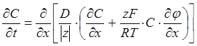
                            ¶C/¶t  =  ¶(D∙¶C/¶x) / ¶x  +  ¶(|v_X|∙C) / ¶x – 2 (v_R/r)∙C                                    (13)

 

The next step is simply amazing – further reduction is possible, by substituting Eq. 12 into Eq. 13, and noting that

 

                            ¶(|v_X|∙C)/ ¶x – 2 (v_R/r)∙C  =  |v_X|∙¶C/¶x + C∙¶|v_X|/¶x – 2 (v_R/r)∙C

                                                                                                =   |v_X|∙¶C/¶x                           (14)

 

Thus the final partial differential equation reduces to the well-known form

 

 

Eq. 15 is quite remarkable for all the cancellations in its derivation.  Although we have assumed both radial and axial flow in the continuity equation, and specifically considered v_x not to be a constant in x in the thin aqueous boundary layer, v_R drops out in the treatment, as does the spatial derivative of v_x (Eq. 14).

 

Additionally, note that we do not assume D to be constant in the aqueous boundary layer.  The Vinograd-McBain electric field treatment (below) addresses the spatial dependence of diffusivity, as a function of all ions present in solution, and especially sensitive to bulk solution pH changes.

 

 

Spinning Disk Fluid Velocity

 

The flow due to a disk rotating in a viscous fluid was originally solved by von Kármán in 1921, and later substantially refined by Cochran in 1934.  More recent discussions may be found in the classic books by Levich,³¹ Cussler,³² and Schlichting and Gersten,³³ and in research papers.^30,34,35,47

 

The tangential, radial, and axial velocity equations, as functions of the distance from the surface of a rotating disk, are summarized in Table 2.  Figure 2 illustrates these fluid velocity profiles as a function of the distance from the surface of the rotating disk, at 200, 400, and 600 RPM, assuming the disk surface area to be 0.3 cm² (radius = 0.309 cm).

 

 

Table 2.  Spinning Disk Fluid Velocity (cm∙s^-1) Equations ^a

 ^a The speed of rotation, w (rad∙s^-1), is obtained by multiplying the RPM value by p/30.  The kinematic viscosity of water, n, is 0.008929 cm²∙s^-1 at 25^oC and 0.0069711 cm²∙s^-1 at 37^oC.  Note 2v_R  = -r∙dv_X/dx. 

 

 

Vinograd-McBain Treatment of Diffusion of Electrolytes and of the Ions in their Mixture

 

Electric fields, created in solutions containing ions migrating under spatial concentration and electrical field gradients, can act on each ion to either retard or accelerate its diffusion velocity from the value the ion would have in the absence of the gradients.  If a solution contains a highly mobile ion, like H⁺, and a sluggish ion, like ClO₄^–, and there is a concentration gradient, the faster ion has the innate tendency to migrate ahead of the slower ion, which creates a charge separation.  Resistance to the latter results in lowered diffusivity of the fast ion and raised diffusivity of the slow one, so that very quickly both ions travel at the same steady-state velocity, in order to maintain spatial charge neutrality.  For example, the diffusivity of H⁺ in a dilute salt solution can be as low as 10 x 10^–6 cm² s^–1 (see below).  However, in a solution containing 0.1 M KCl, the diffusivity of hydrogen ions increases to its non-gradient value of 93 x 10^–6 cm² s^–1.  This needs to be considered in the analysis of dissolution experiments, especially if the ionic strength of the solution is low.  The diffusivity of ions in the ABL can change throughout the layer. This is generally neglected, presumably due to its mathematical complexity. In µDISS-X, these diffusivity shifts are handled automatically, as described by Vinograd-McBain.⁶

 

From the Nernst theory of diffusion of ions, one can solve the partial differential equations (one for each ion), which describe transport of mass under the conditions of electric field and concentration gradients,

                                                                                               (16)

 

 

where z is the valence of the ion, F is the Faraday constant (96486.7 coul mol^–1), ¶j/¶x is the electric potential.   By imposing the electrical neutrality condition for the ion mixture, Vinograd-McBain derived from Eq. 16 the expression for the resultant diffusivity for a given ion, D_j(x), as a fraction of the diffusivity that the ion would have in the absence of concentration gradients and electric fields, D_j*(x),

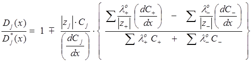                                    (17)

 

 

 

 

where the ‘-’ sign in ‘’ is used if the species j is a cation, and the ‘+’ used if it is an anion.  The summations are taken over all ions present in solution.  The equivalent conductances of cations and anions, l^o₊ and l^o_– , respectively, are in units of W^–1∙cm∙equiv^–1.  Values for common ions at 25^oC: 349.82 (H⁺), 198.5 (OH^–), 73.52 (K⁺), 50.11 (Na⁺), and 76.34 (Cl^–).  For drugs in the ionic state, it can be assumed that l^o_± = D₀ ∙|z_±|∙F² /RT, where D₀ is the diffusivity of the uncharged drug species.  For example, indomethacin at 25^oC has a measured¹⁸ D₀ = 5.6 x 10^-6 cm² s^–1; the corresponding l^o_– = 21.0 W^–1∙cm∙equiv^–1.  Hydrochlorothiazide, with a D₀ = 5.5 x 10^–6 cm² s^–1 (25^oC), is expected to have the corresponding l^o_– = 20.7 and l^o_2– = 41.4 W^–1∙cm∙equiv^–1.

 

Consider the example of indomethacin dissolution, with no background electrolyte added, with stirring at 600 RPM.  For the parameters taken from Mooney et al.,¹⁸ at pH_bulk = 7, the calculated (µDISS-X) concentrations and concentration gradients at x = 0  are: C_H = 9.75 x 10^–6 M, dC_H/dx = –5.15mM/cm, C_A = 9.72 x 10^–6 M, dC_A/dx = –5.15 mM/cm, C_OH    = 1.05 x 10^–9 M, dC_OH/dx = 0.00055 mM/cm, C_K = dC_K/dx = 0, and C_Cl = 4.07 x 10^–8 M (Cl^– comes from HCl titrant added to adjust bulk pH in the sample-free vessel), and dC_Cl/dx = 0.  The expression in the braces in Eq. 17 evaluates to –4.67 x 10⁺⁵.  If the diffusivity of the hydrogen ion in the absence of concentration gradients is 93.2 x 10^–6 cm² s^-1, then the apparent diffusivity value drops to 10.6 x 10^–6 cm² s^–1 in the absence of background electrolyte, as the value in the braces in Eq. 17 is multiplied by C_H/(dC_H/dx) and the result subtracted from 1, according to Eq. 17.  Under these same conditions, the diffusivity of A^– rises to 10.5 x 10^–6 cm² s^–1 (from a value of 5.6 x 10^–6 cm² s^–1) and that of OH^– drops to 6.0 x 10^–6 cm² s^–1 (from a value of 52.9 x 10^–6 cm² s^–1).  In this example, A^– and H⁺ are electrically coupled to travel nearly with the same velocity, in order to maintain electroneutrality.

 

The shifts in the diffusivity coefficients are less dramatic when background salt is added.  For example, for [KCl] = 0.1 M, with pH_bulk = 2.00, the diffusivity of H⁺ drops to 72.5 x 10^–6 cm² s^–1.  (That of A^– is not affected by pH_bulk values.)  At higher pH_bulk values, when indomethacin starts to ionize, diffusivities return to their zero-gradient values.  The coupling between A^– and H⁺ is relaxed by the K⁺ and Cl^– ions from the “swamping” level of background electrolyte.  Such changes in diffusivities as a function of the ion concentrations and concentration gradients in solution are automatically adjusted in µDISS-X.

 

 

Convective Diffusion with Chemical Reaction (CDR)

 

In a dissolution experiment, once an ionizable substance dissolves and begins to diffuse across the ABL, it may undergo chemical reactions at the same time, such as ionization, complexation, micelle formation, excipient interaction, etc. The derivation of the convective diffusion expression, Eq. 15, does not specifically consider this effect.  But, there is a way around this shortfall.  It was shown by Olander³⁶ that if the differential equations for each species are combined to express total concentrations of sample and hydrogen excess, the reaction terms cancel out.  This is a valid procedure, provided the reactions are reversible and fast compared to diffusion. 

 

Mass Balance Considerations

 

As an example to illustrate the Olander “trick,” consider the possible chemical reactions of a diprotic substance, such as hydrochlorothiazide, denoted, AH₂.

 

                        H⁺ + A^2–    D  AH^–                      ß₁₁ = [AH^–] / [A^2–] [H⁺]                                        (18a)

                        2H⁺ + A^2–  D   AH₂                     ß₁₂ = [AH₂] / [A^2–]² [H⁺]                                      (18b)

 

There is also the water ionization reaction, described by the ion-product constant, K_w = [H⁺][OH^–]._.  (The water ion-product depends on ionic strength and temperature: at 25^oC and 0.5 M, K_w = 1.84 x 10^–14 M²; at 0.1 M the value diminishes slightly to 1.63 x 10^–14; at 37^oC and 0.5 M, the value rises to 4.07 x 10^–14.  These changes impact on pH > 7 calculations.³⁷) Equilibrium expressions can be treated in terms of two types of components: (a) “reactants” (e.g., A^2– and H⁺) and (b) "associated species" constructed from reactants (e.g., AH^– and AH₂).³⁸ The hydroxide ion is treated as a form of the hydrogen ion, through the K_w expression, and is not treated as an independent reactant. Note that on the left side of the above expressions we have only primary reactants and on the right side, only associated species.  If the two equilibrium constants for Eqs. 18 are denoted as ß₁₁ and ß₁₂, respectively, then the concentrations of the associated species are [AH^–] = ß₁₁ [A^2–] [H⁺] and [AH₂] = ß₁₂ [A^2–] [H⁺]².  The subscripts 11 and 12 refer to the stoichiometric coefficients of the associated species, in the order A, then H.  Note that the cumulative association constants ß₁₁ = K_a2^-1 and ß₁₂ = (K_a1K_a2)^-1, where K_a1 and K_a2 are normally defined in terms of stepwise dissociation of protons. 

 

The law of mass action links the ionization constants to the calculated concentrations of the reactants and the associated species.  This relationship is usually expressed as a series of mass balance equations, one equation for each reactant (including the hydrogen).  These equations account for all of the reactants as they are apportioned in the various associated species.  In the present example, there are two total concentrations to consider, for which the mass balance equations are

 

                                     [A]_total  =  [A^2–] + [AH^–] + [AH₂]                                                               (19a)

                                     [H]_total  =  [H⁺] – [OH^–] + [AH^–] + 2 [AH₂]                                                  (19b)

 

Substituting the expressions for ß₁₁ and ß₁₂ into Eqs. 19, and defining A = [A]_total, H = [H]_total,  a = [A^2-] and h = [H⁺], produces

 

                                    A  =  a + a h ß₁₁ + a h² ß₁₂                                                                      (20a)

                                    H  =  h – K_w / h + a h ß₁₁ + 2 a h² ß₁₂                                                       (20b)

 

which are polynomials linear in a and cubic in h.  If ß₁₁ and ß₁₂ are known, and A and H represent the sample concentration and hydrogen excess concentration, then the polynomials can be solved for a and h.  Mooney et al.¹⁸ and McNamara et al.^22,23 solved similar expressions to determine the speciation of simple monoprotic acids and bases.  However, for several (multiprotic) reactants Y, Z, …, H,  it is not practical to solve these equations in a closed form with the roots expressed as a function of total concentrations and the ionization constants.  Instead, Newton's method can be used for the more complex cases.^33,34,48  For the general equilibrium expression corresponding to the formation of j^th associated species, one may write

 

                                     e_yj Y  +  e_zj Z  +   e_hj H    D   Y_eyj Z_ezj H_ehj                                               (21)

 

where e_ij is the stoichiometric coefficient for the i^th reactant in the j^th associated species.  The concentration of the j^th species can be stated as

 

                                     C_j  =  y ^eyj z ^ezj h ^ehj ß_j                                                                           (22)

 

Now the ß subscript is simply the associated species index, j, rather than the stoichiometric coefficients.  The mass balance equations for the three-reactant general case can be stated as

 

                                     Y  =  y  +  S_j^N e_yj C_j                                                                              (23a)

                                     Z  =  z  +  S_j^N e_zj C_j                                                                              (23b)

                                     H  =  h   – K_w / h+  S_j^N e_hj C_j                                                                 (23c)

 

where N is the total number of associated species, Y and Z are the total concentrations, y and z are the concentrations of the reactants.  The method to solve Eqs. 23 for y, z, and h calls for the evaluation of the partial derivatives (¶Y/¶pY), (¶Z/¶pY), (¶H/¶pY), (¶Y/¶pZ), (¶Z/¶pZ), (¶H/¶pZ),  (¶Y/¶pH), (¶Z/¶pH), and (¶H/¶pH), using analytical expressions.^38,39,48  A symmetric matrix of these derivatives, called the Jacobian matrix, is inverted; pY (= –log[Y]), pZ, and pH are iteratively refined to convergence.^39-43,48,49

 

Olander³⁶ showed that if one takes Eq. 15 for each reactant (e.g., in the two-reactant diprotic acid example) and combines the equations into the mass balance form along the lines of Eqs. 19, the chemical reaction terms cancel out, and the two total concentration differentials become

 

           ¶A/¶t  =  ¶(D_H2A∙¶C_H2A/¶x)/¶x  +  ¶(D_HA∙¶C_HA/¶x)/¶x  +  ¶(D_A∙¶C_A/¶x)/¶x

                             +  |v_X|∙¶A/¶x                                                                                              (24a)

           ¶H/¶t  =  ¶(D_H∙¶C_H/¶x)/¶x  –  ¶(D_OH∙¶C_OH/¶x)/¶x +  ¶(D_HA∙¶C_HA/¶x)/¶x

                             + 2  ¶(D_H2A∙¶C_H2A/¶x)/¶x  + |v_X|∙¶H/¶x                                                          (24b)

 

The solution of Eqs. 24 for the total concentrations A and H, concomitant with the computation of all reactant and associated species, is central to the µDISS-X method. 

 

 

Analytical Solution to the Convective Diffusion with Chemical Reaction Equations    

Cussler³² and Pohl and coworkers^45,46 described the solution of Eq. 15, assuming a single and constant diffusivity and thickness of the aqueous boundary layer (without explicit consideration of chemical reactions), under steady state condition:

 

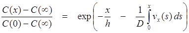                                                                   (25)

 

To demonstrate that the numerical solution to the convective diffusion equation yields Eq. 26, we fitted the total concentration curve arising from the numerical equation in the steady-state limit (t >  0.4 s), to a parameterized form of Eq. 25, with v_x(x) taken from Table 2:

                    

 

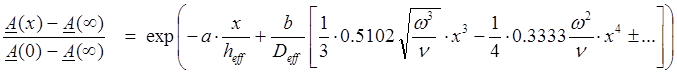
(26)

 

where a and b are adjustable parameters, with the expectation values of unity.  In the regression analysis of Eq. 26, the effective “total” diffusivity, D_eff, was approximated to be that of the neutral species,

 

                                                                                                  

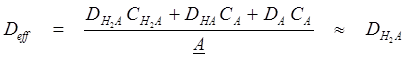
(27)

 

The “effective” thickness of the aqueous boundary layer, h_eff, is not constant in principle, since according to the Levich³¹ equation,

 

                                                                                                        (28)

 

the diffusivity of the species can affect the ABL thickness.  In Eq. 26, we approximated h_eff by assuming a single D_eff, from Eq. 27.  Eq. 26 was fitted to the steady-state concentration curve calculated by the numerical method.  The refined parameters were a = 1.0444 and b = 1.0966 (r² = 0.9999, SD = 0.004, F = 70764,   n = 81).  Both are very close to 1, and suggest that the numerical solution agrees closely to that obtained by the analytical method, as illustrated in Figure 3 (points = numerical solution, solid curve = analytical solution, dashed line = the tangent curve at x = 0, intersecting the x-axis at x = h).

 

The deviation of a and b from exact unit values may be due to our taking into account the spatial dependence of diffusivity coefficients (Vinograd-McBain method) in the ABL during the numerical procedure, whereas D_eff in Eq. 27 is simply taken to be that of the neutral species.   To a lesser detriment, a single thickness of the ABL is implied by Eq. 26, set equal to that of the neutral species.  (This surely will need to be questioned, when large micelles are used as excipients in the simulation study.)

 

Hence, a little bit is given up in rigor in the numerical-analytical “calibration.”  The overwhelming gain in using Eq. 26 is speed of calculation, which simply cannot be matched by the robust and versatile, but extremely slow numerical procedure.

 

Using Eq. 26, we are able to calculate the total sample concentration at any point in the ABL, without prior knowledge of the underlying equilibrium model.  Having the total concentrations at any value of x, hence, can be the starting point to calculate the entire speciation, by solving the static mass balance equations like Eqs. 20 or 23, a task for which µDISS-X is particularly well suited.

 

 

DISSOLUTION OF SPHERICAL PARTICLES IN A STIRRED SOLUTION

 

 

Theory

 

So far, we have considered dissolution of compounds from rotating planar surfaces, where, at steady state, the classical Nernst-Brünner thin-film model predicts a linear decrease in concentration of the dissolving species throughout the aqueous boundary layer (ABL).  With a spherical particle, on the other hand, the concentration gradient is not linear in the ABL, but decreases with distance from the surface of the particle.  Figure 4 shows the nonlinear relationships for several particle sizes. Dissolution of a spherical surface will not reach a conventional steady state, because the surface area continually changes with time, as the dissolving particles shrink in size.

 

The most common expression used to describe the dissolution of a spherical particle follows the so-called “cube-root law,” ⁴⁴

 

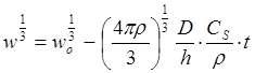                                                                                                 (29)

 

where w is the weight (g) of the particle at time t, w_o is the starting weight, r is the density of the solid (g cm^-3), and C_S is the solubility (g cm^-3). 

 

Wang and Flanagan^7,8 discussed this and other similar particle dissolution equations, and found that the equations were only approximate, since assumptions made in their derivations were not valid under broad range of practical conditions.  These investigators proceeded to derive a general model for diffusion-controlled particle dissolution. 

 

Consider a spherical particle with a radius a (a_o at t=0) and the ABL surrounding it with a thickness of h.  In spherical coordinates, the ABL extends isotropically from r = a to r = a+h.  Wang and Flanagan defined a practical pseudo steady state condition, where mass transport rates across the inner (r = a) and outer (r = a+h) spherical surfaces are assumed to be equal.  That is, within the time for a molecule to cross the ABL, the surface area is essentially unchanged.  This assumption was central to their subsequent derivations.

 

Under sink conditions, Wang and Flanagan⁷ derived

                                           

 

 

 

 

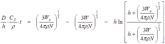
(30)

 

where W stands for the total weight of N particles.  Comparisons of Eq. 29 to 30, suggested that Eq. 29 is a special case of Eq. 30, where the radius of the particle is much larger than the thickness of the ABL (a >> h). The investigators also derived the non-sink equation accompanying Eq. 30.  Their very complicated equation (not reproduced here) has been incorporated into µDISS-X.  

 

 

Application of Wang-Flanagan Model to the Dissolution of 2-Naphthoic Acid and Phenazopyridine Hydrochloride, as Powders of Known Particle Size Distribution

 

The small-volume dissolution apparatus (mDISS Profiler from pION INC) was used to measure the dissolution rates of powders of 2-naphthoic acid and phenazopyridine hydrochloride.  The particulate properties of the two powders were independently determined: the specific surface area of 2-naphthoic acid and phenazopyridine hydrochloride were determined to be 0.34 and 1.31 m²∙g^–1, respectively; particles were mainly in the 10 –20 mm (38% of 2-naphthoic acid and 25% of phenazopyridine.HCl) and 20 – 40 mm (28% of 2-naphthoic acid and 39% of phenazopyridine hydrochloride).  In the µDISS-X simulation calculations, the average sizes of particles were taken as 21 mm (2-naphthoic acid) and 24 mm (phenazopyridine.HCl).

 

About 1 mg of 2-naphthoic acid was weighed into each of eight sample tubes.  This is a very low consumption of the API, much lower than the traditional disk-IDR methods.  To each, 20 mL of pH 7.4 buffer (0.05 M HEPES), was added, and magnetically stirred at 700 RPM.  In about 20 min, the weak acid dissolution reached a steady state.  Simulations indicated that at pH 7.4, in the presence of a high capacity buffer, the weak acid test compound dissolved completely.  This was visually confirmed.

 

The case of phenazopyridine.HCl was more complex than that of the weak acid.  Only about 0.75 ± 0.04 mg of the hydrochloride salt of the weak base was weighed into each of eight test tubes of the Profiler apparatus.  As before, to each, 20 mL of pH 7.4 buffer was added, and the stirring rate was set to 700 RPM.  The thermodynamic calculation by µDISS-X predicted that the solid, introduced as a powder in the form of the hydrochloride salt, should undergo a transformation into the free base solid at pH 7.4.  This must be a very fast conversion, since the observed rate is comparable to that of the dissolution of free base solid, if Figure 5 is any guide. 

 

The observed maximum flux at the start of the dissolution experiment was about 7.4 x 10 ^–10 mol∙cm^–2∙s^–1, based on the estimated total surface area of 1.34 cm² (A = 3 w/(a_or), where w = 0.00075 g, a_o = 1.2 x 10^-3 cm radius particles of density, r = 1.4 g∙cm^–3).  The experimentally determined specific surface area, 1.31 m² g^–1, suggests a higher total surface area of 9.80 cm², and thus a lower initial flux of 1.0 x 10 ^–10 mol∙cm^‑2∙s^–1.  The calculated initial flux, based on the Wang-Flanagan model, is 6.0 x 10 ^–10 mol∙cm^–2∙s^–1, assuming 12 mm particle radius, solid density = 1.4 g cm^–3, and D = 6.4 x10 ^–6 cm²∙s^–1.

 

The dissolution reached a steady state in about 8 hr.  Simulations indicate that at pH 7.4, adjusted with the 0.05 M buffer, phenazopyridine is not completely dissolved.  This was confirmed visually.  Figure 6 shows the six traces of the salt dissolution curves, as well as the calculated dissolution curve.  The concentration–time profile was calculated by the Profiler processing software (pION INC), based on the area under the second-derivative curves (optical density vs. wavelength) in the wavelength interval 322 to 360 nm, a strategy minimizing the contributions due to the background scattering of the turbid solutions. The Wang-Flanagan model correctly predicted the time course of the dissolution of the powder, when the experimental surface area is calculated based on the average radius of assumed spherical particles.

 

After about 18 hr, the concentrations in each of the vessels level off to a constant value of 15.1 ± 0.6 mg∙mL^-1, very close to the 14.5 mg∙mL^-1 solubility determined independently by the “self-calibrating” microtitre plate UV method.¹⁰

 

It is interesting to note that if more sample had been used, e.g., 750 mg of phenazopyridine hydrochloride, rather than 0.75 mg, the phenazopyridine.HCl solubility product would have been exceeded.  There would have been enough compound to form coprecipitates of the free base and the hydrochloride salt.  Under this condition of the Gibbs “super buffer,” the interfacial pH is predicted to drop to 3.14 (from a value slightly below pH 7.4 in the 0.75 mg case), and the flux to increase by more than 100 fold.  The equilibration time would drop from about 20 hr to less than 1 hr.  However, this rapid rate of dissolution would only be maintained under excessive amount of compound.  As the dissolution process decreases the weight of solid below the solubility product limit, then a slower dissolution mechanism would prevail.

 

 

REFERENCES

 

1. Avdeef, A. Absorption and Drug Development; Wiley-Interscience: New York, 2003; pp116-246.

2. Grant, DJW, Higuchi T.  Solubility Behavior of Organic Compounds; John Wiley & Sons: New York, 1990; pp 385-388,474-486.

3. Anderson BD, Flora KP. Preparation of water-soluble compounds through salt formation. In The Practice of Medicinal Chemistry; Wermuth, C.G. , Ed.; Academic Press: London, 1996; pp 739-754.

4. McNamara DP, Vieira ML, Crison JR.  Dissolution of pharmaceuticals in simple and complex systems.  In Transport Processes in Pharmaceutical Systems; Amidon, G.L.; Lee, P.I.; Topp, E.M. , Eds.; Marcel Dekker, Inc.: New York, 2000; pp 109-146.

5. Streng WH.  Characterization of Compounds in Solution – Theory and Practice.  Kluwer Academic: New York, 2001; pp 61-218.

6. Vinograd JR, McBain JW.  Diffusion of electrolytes and of the ions in their mixture. J. Amer. Chem. Soc. 1941, 63, 2008-2015.

7. Wang J, Flanagan DR.  General solution for diffusion-controlled dissolution of spherical particles. 1. Theory.  J. Pharm. Sci. 1999, 88, 731-738.

8. Wang J, Flanagan DR.  General solution for diffusion-controlled dissolution of spherical particles. 1. Evaluation of experimental data. J. Pharm. Sci. 2002, 91, 534-542.

9. Avdeef A, Voloboy D, Foreman A.  Dissolution and solubility.  In: Testa B, van de Waterbeemd H (eds.). Comprehensive Medicinal Chemistry II, Elsevier: Oxford, UK, 2007, pp. 399-423. 

10. Avdeef A. Solubility of sparingly-soluble drugs. Dressman J, Reppas C. (eds., special issue: The Importance of Drug Solubility).  Adv. Drug Deliv. Rev. 2007, 59, 568-590.

11. Avdeef A, Tsinman O.  Miniaturized rotating disk intrinsic dissolution rate measurement: effects of buffer capacity in comparisons to traditional Wood’s apparatus. Pharm. Res. 2008, 25, 2613-2627.

12. Tsinman K, Avdeef A, Tsinman O, Voloboy D. Powder dissolution method for estimating rotating disk intrinsic dissolution rates of low solubility drugs. Pharm. Res. 2009, 26, 2093-2100.

13. Avdeef A, Tsinman K, Tsinman O, Sun N, Voloboy D. Miniaturization of powder dissolution measurement and estimation of particle size. Chem. Biodiv. 2009,11, 1796-1811.

14.  Fagerberg JH, Tsinman O, Tsinman K, Sun N, Avdeef A, Bergström CAS.  Dissolution Rate and Apparent Solubility of Poorly Soluble Compounds in Biorelevant Dissolution Media. Mol. Pharmaceutics 2010, 7, 1419-1430.

15. Higuchi, W.; Parrot, E.L.; Wurster, D.E.; Higuchi, T.  Investigation of drug release from solids. II. Theoretical and experimental study of influences of bases and buffers on rates of dissolution of acidic solids.  J. Amer. Pharm. Assoc. 1958, 47, 376-383. 

16. Higuchi, T.; Shih, F.-M.L.; MKimura, T.; Rytting, J.H.  Solubility Determination of Barely Aqueous Soluble Organic Solids.  J. Pharm. Sci. 1979, 68, 1267-1272.

17. Mooney, K.G.  Dissolution Kinetics of Organic Acids. Ph.D. Dissertation, University of Kansas, 1980.

18. Mooney, K.G.; Mintun, M.A.; Himmelstein, K.J.; Stella, V.J.  Dissolution Kinetics of Carboxylic Acids. I: Effect of pH under Unbuffered Conditions.  J. Pharm. Sci. 1981, 70, 13-22.

19. Mooney, K.G.; Mintun, M.A.; Himmelstein, K.J.; Stella, V.J.  Dissolution Kinetics of Carboxylic Acids. II: Effects of Buffers.  J. Pharm. Sci. 1981, 70, 22-32.

20. Mooney, K.G.; Rodriguez-Gaxiola, M.; Mintun, M.; Himmelstein, K.J.; Stella, V.J.  Dissolution Kinetics of phenylbutazone. J. Pharm. Sci. 1981, 70, 1358-1365.

21. McNamara, D.P.  Dissolution of acidic and basic compounds from a rotating disk. Influences of diffusion, convection and reaction.  Ph.D. Dissertation, University of Michigan, 1986.

22. McNamara, D.P.; Amidon, G.L.   Dissolution of acidic and basic compounds from the rotating disk: influence of convective diffusion and reaction.  J. Pharm. Sci. 1986, 75, 858-868.

23. McNamara, D.P.; Amidon, G.L.  Reaction plane approach for estimating the effects of buffers on the dissolution rate of acidic drugs.  J. Pharm. Sci. 1988, 77, 511-517.

24. Southard, M.Z.; Green, D.W.; Stella, V.J.; Himmelstein, K.J.  Dissolution of ionizable drugs into unbuffered solution: a comprehensive model for mass transport and reaction in the rotating disk geometry.  Pharm. Res. 1992, 9, 58-69.

25. Wood, J.H.; Syarto, J.E.; Letterman, H. Improved holder for intrinsic dissolution rate studies.  J. Pharm. Sci. 1965, 54, 1068-.

26. Noyes, A.A.;  Whitney, W.R.  The rate of solution of solid substances in their own solutions.   J. Amer. Chem. Soc. 1897, 19, 930-934.

27. Brünner, E.  Reaktionsgeschwindigkeit in heterogenen systemen.  Z. Phys. Chem. 1904, 47, 56-102.

28. Nernst, W.  Theorie der reaktionsgeschwindigkeit in heterogenen systemen.  Z. Phys. Chem.1904, 47, 52-55.

29. Weiss, T.F.  Cellular Biophysics, Vol. 1, MIT Press: Cambridge, MA, 1996; p 124.

30. Litt, M.; Serad, G.  Chemical reactions on a rotating disk. Chem. Eng. Sci. 1964, 19, 867-884.

31. Levich, V.G. Physiochemical Hydrodynamics; Prentice-Hall: Englewood Cliffs, N.J., 1962; pp 39-72.

32. Cussler, E.L. Diffusion – Mass Tranfer in Fluid Systems, 2^nd ed.; Cambridge Univ. Press: Cambridge, 1997; pp 70-72.

33. Schlichting, H.; Gersten, K.  Boundary Layer Theory, 8^th ed.; Springer-Verlag: Berlin, 2000; pp 119-124, 328-330, 483-485.

34. Kelson, N.; Desseaux, A.  Note on porous rotating disk flow.  ANZIAM J.  2000, 42, C837-C855.

35. Miklav…i…, M.; Wang, C.Y.  The flow due to a rough rotating disk. Z. angew. Math. Phys. 2004, 54, 1-12.

36. Olander, D.R.  Simultaneous mass transfer and equilibrium chemical reaction.  A.I.Ch.E. J. 1960, 6, 233-239.

37. Sweeton, F.H.; Mesmer, R.E.; Baes, C.F. Jr.  Acidity measurements at elevated temperatures. 7. Dissociation of water.  J. Solut. Chem. 1974, 3, 191-214. 

38. Avdeef, A.  STBLTY: Methods for Construction and Refinement of Equilibrium Models. In Computational Methods for the Determination of Formation Constants; Leggett, D.J., Ed.; Plenum Press: New York, 1985; pp 355-474.

39. Avdeef, A.; Raymond, K.N. Free metal and free ligand concentrations determined from titrations using only a pH electrode.  Partial derivatives in equilibrium studies.  Inorg. Chem. 1979, 18, 1605-1611.

40. Avdeef, A.;  Zelazowski, A.Z.; Garvey, J.S. Cadmium binding by biological ligands. 3. Five- and seven-cadmium binding in metallothionein: a detailed thermodynamic study.  Inorg. Chem. 1985, 24, 1928-1933

41. Avdeef, A.  Weighting Scheme for Regression Analysis Using pH Data from Acid-Base Titrations.  Anal. Chim. Acta 1983, 148, 237-244.

42. Avdeef, A.  pH-Metric log P. II: Refinement of partition coefficients and ionization constants of multiprotic substances.  J. Pharm. Sci. 1993, 82, 183-190.

43. Avdeef, A.; Bucher, J.J.  Accurate measurements of the concentration of hydrogen ions with a glass electrode: calibrations using the Prideaux and other universal buffer solutions and a computer-controlled automatic titrator.  Anal. Chem. 1978, 50, 2137-2142.

44. Press, W.H.; Teukolsky, S.A.; Vetterling, W.T.; Flannery, B.P.  Numerical Recipes in C – The Art of Scientific Computing, 2^nd ed.; Cambridge Univ. Press: Cambridge, 1992, pp 827-851.

45. Pohl, P.; Saparov, S.M.; Antonenko, Y.N. The effect of a transmembrane osmotic flux on the ion concentration distribution in the immediate membrane vicinity measured by microelectrodes.  Biophys. J. 1997, 72, 1711-1718.

46. Pohl, P.; Saparov, S.M.; Antonenko, Y.N.  The size of the unstirred layer as a function of the solute diffusion coefficient.  Biophys. J. 1998, 75, 1403-1409.

47. Hixson, A.W.; Crowell, J.H. Dependence of reaction velocity upon surface and agitation. I. Theoretical considerations. Ind. Eng. Chem.1931, 23, 923-931.

48. Avdeef, A.  pH-Metric Solubility. 1. Solubility-pH Profiles from Bjerrum Plots. Gibbs Buffer and pK_a in the Solid State.  Pharm. Pharmacol. Commun. 1998, 4, 165-178.

49. Avdeef, A.; Berger, C.M.  pH-Metric Solubility. 3.  Dissolution titration template method for solubility determination. Eur. J. Pharm. Sci. 2001, 14, 281-291.